Descriptive Statistics | Definitions, Types, Examples
Descriptive statistics summarize and organize characteristics of a data set. A data set is a collection of responses or observations from a sample or entire population.
In quantitative research, after collecting data, the first step of statistical analysis is to describe characteristics of the responses, such as the average of one variable (e.g., age), or the relation between two variables (e.g., age and creativity).
The next step is inferential statistics, which help you decide whether your data confirms or refutes your hypothesis and whether it is generalizable to a larger population.
Types of descriptive statistics
There are 3 main types of descriptive statistics:
- The distribution concerns the frequency of each value.
- The central tendency concerns the averages of the values.
- The variability or dispersion concerns how spread out the values are.
You can apply these to assess only one variable at a time, in univariate analysis, or to compare two or more, in bivariate and multivariate analysis.
- Go to a library
- Watch a movie at a theater
- Visit a national park
Your data set is the collection of responses to the survey. Now you can use descriptive statistics to find out the overall frequency of each activity (distribution), the averages for each activity (central tendency), and the spread of responses for each activity (variability).
Frequency distribution
A data set is made up of a distribution of values, or scores. In tables or graphs, you can summarize the frequency of every possible value of a variable in numbers or percentages.
| Gender | Number |
|---|---|
| Male | 182 |
| Female | 235 |
| Other | 27 |
From this table, you can see that more women than men or people with another gender identity took part in the study.
| Library visits in the past year | Percent |
|---|---|
| 0–4 | 6% |
| 5–8 | 20% |
| 9–12 | 42% |
| 13–16 | 24% |
| 17+ | 8% |
From this table, you can see that most people visited the library between 5 and 16 times in the past year.
Measures of central tendency
Measures of central tendency estimate the center, or average, of a data set. The mean, median and mode are 3 ways of finding the average.
Here we will demonstrate how to calculate the mean, median, and mode using the first 6 responses of our survey.
The mean, or M, is the most commonly used method for finding the average.
To find the mean, simply add up all response values and divide the sum by the total number of responses. The total number of responses or observations is called N.
| Data set | 15, 3, 12, 0, 24, 3 |
|---|---|
| Sum of all values | 15 + 3 + 12 + 0 + 24 + 3 = 57 |
| Total number of responses | N = 6 |
| Mean | Divide the sum of values by N to find M: 57/6 = 9.5 |
The median is the value that’s exactly in the middle of a data set.
To find the median, order each response value from the smallest to the biggest. Then, the median is the number in the middle. If there are two numbers in the middle, find their mean.
| Ordered data set | 0, 3, 3, 12, 15, 24 |
|---|---|
| Middle numbers | 3, 12 |
| Median | Find the mean of the two middle numbers: (3 + 12)/2 = 7.5 |
The mode is the simply the most popular or most frequent response value. A data set can have no mode, one mode, or more than one mode.
To find the mode, order your data set from lowest to highest and find the response that occurs most frequently.
| Ordered data set | 0, 3, 3, 12, 15, 24 |
|---|---|
| Mode | Find the most frequently occurring response: 3 |
Measures of variability
Measures of variability give you a sense of how spread out the response values are. The range, standard deviation and variance each reflect different aspects of spread.
Range
The range gives you an idea of how far apart the most extreme response scores are. To find the range, simply subtract the lowest value from the highest value.
Range: 24 – 0 = 24
Standard deviation
The standard deviation (s) is the average amount of variability in your dataset. It tells you, on average, how far each score lies from the mean. The larger the standard deviation, the more variable the data set is.
There are six steps for finding the standard deviation:
- List each score and find their mean.
- Subtract the mean from each score to get the deviation from the mean.
- Square each of these deviations.
- Add up all of the squared deviations.
- Divide the sum of the squared deviations by N – 1.
- Find the square root of the number you found.
| Raw data | Deviation from mean | Squared deviation |
|---|---|---|
| 15 | 15 – 9.5 = 5.5 | 30.25 |
| 3 | 3 – 9.5 = -6.5 | 42.25 |
| 12 | 12 – 9.5 = 2.5 | 6.25 |
| 0 | 0 – 9.5 = -9.5 | 90.25 |
| 24 | 24 – 9.5 = 14.5 | 210.25 |
| 3 | 3 – 9.5 = -6.5 | 42.25 |
| M = 9.5 | Sum = 0 | Sum of squares = 421.5 |
Step 5: 421.5/5 = 84.3
Step 6: √84.3 = 9.18
From learning that s = 9.18, you can say that on average, each score deviates from the mean by 9.18 points.
Variance
The variance is the average of squared deviations from the mean. Variance reflects the degree of spread in the data set. The more spread the data, the larger the variance is in relation to the mean.
To find the variance, simply square the standard deviation. The symbol for variance is s2.
s = 9.18
s2 = 84.3
Univariate descriptive statistics
Univariate descriptive statistics focus on only one variable at a time. It’s important to examine data from each variable separately using multiple measures of distribution, central tendency and spread. Programs like SPSS and Excel can be used to easily calculate these.
| Visits to the library | |
|---|---|
| N | 6 |
| Mean | 9.5 |
| Median | 7.5 |
| Mode | 3 |
| Standard deviation | 9.18 |
| Variance | 84.3 |
| Range | 24 |
If you were to only consider the mean as a measure of central tendency, your impression of the “middle” of the data set can be skewed by outliers, unlike the median or mode.
Likewise, while the range is sensitive to extreme values, you should also consider the standard deviation and variance to get easily comparable measures of spread.
Bivariate descriptive statistics
If you’ve collected data on more than one variable, you can use bivariate or multivariate descriptive statistics to explore whether there are relationships between them.
In bivariate analysis, you simultaneously study the frequency and variability of two variables to see if they vary together. You can also compare the central tendency of the two variables before performing further statistical tests.
Multivariate analysis is the same as bivariate analysis but with more than two variables.
Contingency table
In a contingency table, each cell represents the intersection of two variables. Usually, an independent variable (e.g., gender) appears along the vertical axis and a dependent one appears along the horizontal axis (e.g., activities). You read “across” the table to see how the independent and dependent variables relate to each other.
| Number of visits to the library in the past year | |||||
|---|---|---|---|---|---|
| Group | 0–4 | 5–8 | 9–12 | 13–16 | 17+ |
| Children | 32 | 68 | 37 | 23 | 22 |
| Adults | 36 | 48 | 43 | 83 | 25 |
Interpreting a contingency table is easier when the raw data is converted to percentages. Percentages make each row comparable to the other by making it seem as if each group had only 100 observations or participants. When creating a percentage-based contingency table, you add the N for each independent variable on the end.
| Visits to the library in the past year (Percentages) | ||||||
|---|---|---|---|---|---|---|
| Group | 0–4 | 5–8 | 9–12 | 13–16 | 17+ | N |
| Children | 18% | 37% | 20% | 13% | 12% | 182 |
| Adults | 15% | 20% | 18% | 35% | 11% | 235 |
From this table, it is more clear that similar proportions of children and adults go to the library over 17 times a year. Additionally, children most commonly went to the library between 5 and 8 times, while for adults, this number was between 13 and 16.
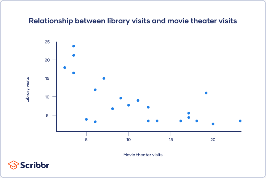
Scatter plots
A scatter plot is a chart that shows you the relationship between two or three variables. It’s a visual representation of the strength of a relationship.
In a scatter plot, you plot one variable along the x-axis and another one along the y-axis. Each data point is represented by a point in the chart.
From your scatter plot, you see that as the number of movies seen at movie theaters increases, the number of visits to the library decreases. Based on your visual assessment of a possible linear relationship, you perform further tests of correlation and regression.
Frequently asked questions about descriptive statistics
- What’s the difference between descriptive and inferential statistics?
-
Descriptive statistics summarize the characteristics of a data set. Inferential statistics allow you to test a hypothesis or assess whether your data is generalizable to the broader population.
- What are the 3 main types of descriptive statistics?
-
The 3 main types of descriptive statistics concern the frequency distribution, central tendency, and variability of a dataset.
- Distribution refers to the frequencies of different responses.
- Measures of central tendency give you the average for each response.
- Measures of variability show you the spread or dispersion of your dataset.
- What’s the difference between univariate, bivariate and multivariate descriptive statistics?
-
- Univariate statistics summarize only one variable at a time.
- Bivariate statistics compare two variables.
- Multivariate statistics compare more than two variables.
Sources in this article
We strongly encourage students to use sources in their work. You can cite our article (APA Style) or take a deep dive into the articles below.
This Scribbr articleBhandari, P. (October 10, 2022). Descriptive Statistics | Definitions, Types, Examples. Scribbr. Retrieved October 20, 2022, from https://www.scribbr.com/statistics/descriptive-statistics/