Multiple Linear Regression | A Quick Guide (Examples)
Regression models are used to describe relationships between variables by fitting a line to the observed data. Regression allows you to estimate how a dependent variable changes as the independent variable(s) change.
Multiple linear regression is used to estimate the relationship between two or more independent variables and one dependent variable. You can use multiple linear regression when you want to know:
- How strong the relationship is between two or more independent variables and one dependent variable (e.g. how rainfall, temperature, and amount of fertilizer added affect crop growth).
- The value of the dependent variable at a certain value of the independent variables (e.g. the expected yield of a crop at certain levels of rainfall, temperature, and fertilizer addition).
Because you have two independent variables and one dependent variable, and all your variables are quantitative, you can use multiple linear regression to analyze the relationship between them.
Assumptions of multiple linear regression
Multiple linear regression makes all of the same assumptions as simple linear regression:
Homogeneity of variance (homoscedasticity): the size of the error in our prediction doesn’t change significantly across the values of the independent variable.
Independence of observations: the observations in the dataset were collected using statistically valid methods, and there are no hidden relationships among variables.
In multiple linear regression, it is possible that some of the independent variables are actually correlated with one another, so it is important to check these before developing the regression model. If two independent variables are too highly correlated (r2 > ~0.6), then only one of them should be used in the regression model.
Normality: The data follows a normal distribution.
Linearity: the line of best fit through the data points is a straight line, rather than a curve or some sort of grouping factor.
How to perform a multiple linear regression
Multiple linear regression formula
The formula for a multiple linear regression is:

 = the predicted value of the dependent variable
 = the y-intercept (value of y when all other parameters are set to 0)
 = the regression coefficient () of the first independent variable (
 ) (a.k.a. the effect that increasing the value of the independent variable has on the predicted y value)
- … = do the same for however many independent variables you are testing
 = the regression coefficient of the last independent variable
 = model error (a.k.a. how much variation there is in our estimate of )
 = the predicted value of the dependent variable
 = the y-intercept (value of y when all other parameters are set to 0)
 ) of the first independent variable (
 ) (a.k.a. the effect that increasing the value of the independent variable has on the predicted y value)
 = the regression coefficient of the last independent variable
 = model error (a.k.a. how much variation there is in our estimate of
 To find the best-fit line for each independent variable, multiple linear regression calculates three things:
- The regression coefficients that lead to the smallest overall model error.
- The t-statistic of the overall model.
- The associated p-value (how likely it is that the t-statistic would have occurred by chance if the null hypothesis of no relationship between the independent and dependent variables was true).
It then calculates the t-statistic and p-value for each regression coefficient in the model.
Multiple linear regression in R
While it is possible to do multiple linear regression by hand, it is much more commonly done via statistical software. We are going to use R for our examples because it is free, powerful, and widely available. Download the sample dataset to try it yourself.
Dataset for multiple linear regression (.csv)
Load the heart.data dataset into your R environment and run the following code:
heart.disease.lm<-lm(heart.disease ~ biking + smoking, data = heart.data)This code takes the data set heart.data and calculates the effect that the independent variables biking and smoking have on the dependent variable heart disease using the equation for the linear model: lm().
Learn more by following the full step-by-step guide to linear regression in R.

Interpreting the results
To view the results of the model, you can use the summary() function:
summary(heart.disease.lm)This function takes the most important parameters from the linear model and puts them into a table that looks like this:
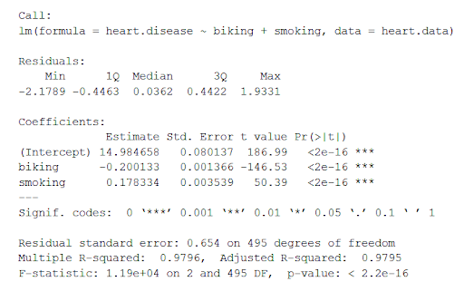
The summary first prints out the formula (‘Call’), then the model residuals (‘Residuals’). If the residuals are roughly centered around zero and with similar spread on either side, as these do (median 0.03, and min and max around -2 and 2) then the model probably fits the assumption of heteroscedasticity.
Next are the regression coefficients of the model (‘Coefficients’). Row 1 of the coefficients table is labeled (Intercept) – this is the y-intercept of the regression equation. It’s helpful to know the estimated intercept in order to plug it into the regression equation and predict values of the dependent variable:
The most important things to note in this output table are the next two tables – the estimates for the independent variables.
The Estimate column is the estimated effect, also called the regression coefficient or r2 value. The estimates in the table tell us that for every one percent increase in biking to work there is an associated 0.2 percent decrease in heart disease, and that for every one percent increase in smoking there is an associated .17 percent increase in heart disease.
The Std.error column displays the standard error of the estimate. This number shows how much variation there is around the estimates of the regression coefficient.
The t value column displays the test statistic. Unless otherwise specified, the test statistic used in linear regression is the t-value from a two-sided t-test. The larger the test statistic, the less likely it is that the results occurred by chance.
The Pr( > | t | ) column shows the p-value. This shows how likely the calculated t-value would have occurred by chance if the null hypothesis of no effect of the parameter were true.
Because these values are so low (p < 0.001 in both cases), we can reject the null hypothesis and conclude that both biking to work and smoking both likely influence rates of heart disease.
Presenting the results
When reporting your results, include the estimated effect (i.e. the regression coefficient), the standard error of the estimate, and the p-value. You should also interpret your numbers to make it clear to your readers what the regression coefficient means.
Visualizing the results in a graph
It can also be helpful to include a graph with your results. Multiple linear regression is somewhat more complicated than simple linear regression, because there are more parameters than will fit on a two-dimensional plot.
However, there are ways to display your results that include the effects of multiple independent variables on the dependent variable, even though only one independent variable can actually be plotted on the x-axis.
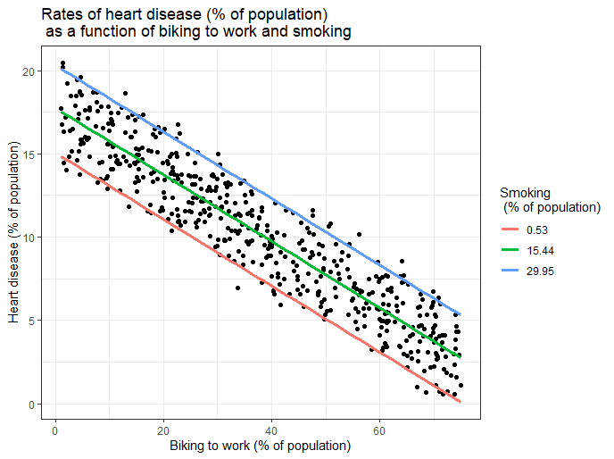
Here, we have calculated the predicted values of the dependent variable (heart disease) across the full range of observed values for the percentage of people biking to work.
To include the effect of smoking on the independent variable, we calculated these predicted values while holding smoking constant at the minimum, mean, and maximum observed rates of smoking.
Frequently asked questions about multiple linear regression
- What is a regression model?
-
A regression model is a statistical model that estimates the relationship between one dependent variable and one or more independent variables using a line (or a plane in the case of two or more independent variables).
A regression model can be used when the dependent variable is quantitative, except in the case of logistic regression, where the dependent variable is binary.
- What is multiple linear regression?
-
Multiple linear regression is a regression model that estimates the relationship between a quantitative dependent variable and two or more independent variables using a straight line.
- How is the error calculated in a linear regression model?
-
Linear regression most often uses mean-square error (MSE) to calculate the error of the model. MSE is calculated by:
- measuring the distance of the observed y-values from the predicted y-values at each value of x;
- squaring each of these distances;
- calculating the mean of each of the squared distances.
Linear regression fits a line to the data by finding the regression coefficient that results in the smallest MSE.
Sources in this article
We strongly encourage students to use sources in their work. You can cite our article (APA Style) or take a deep dive into the articles below.
This Scribbr articleBevans, R. (June 1, 2022). Multiple Linear Regression | A Quick Guide (Examples). Scribbr. Retrieved October 19, 2022, from https://www.scribbr.com/statistics/multiple-linear-regression/
