Two-Way ANOVA | Examples & When To Use It
ANOVA (Analysis of Variance) is a statistical test used to analyze the difference between the means of more than two groups.
A two-way ANOVA is used to estimate how the mean of a quantitative variable changes according to the levels of two categorical variables. Use a two-way ANOVA when you want to know how two independent variables, in combination, affect a dependent variable.
You can use a two-way ANOVA to find out if fertilizer type and planting density have an effect on average crop yield.
When to use a two-way ANOVA
You can use a two-way ANOVA when you have collected data on a quantitative dependent variable at multiple levels of two categorical independent variables.
A quantitative variable represents amounts or counts of things. It can be divided to find a group mean.
A categorical variable represents types or categories of things. A level is an individual category within the categorical variable.
You should have enough observations in your data set to be able to find the mean of the quantitative dependent variable at each combination of levels of the independent variables.
Both of your independent variables should be categorical. If one of your independent variables is categorical and one is quantitative, use an ANCOVA instead.
How does the ANOVA test work?
ANOVA tests for significance using the F-test for statistical significance. The F-test is a groupwise comparison test, which means it compares the variance in each group mean to the overall variance in the dependent variable.
If the variance within groups is smaller than the variance between groups, the F-test will find a higher F-value, and therefore a higher likelihood that the difference observed is real and not due to chance.
A two-way ANOVA with interaction tests three null hypotheses at the same time:
- There is no difference in group means at any level of the first independent variable.
- There is no difference in group means at any level of the second independent variable.
- The effect of one independent variable does not depend on the effect of the other independent variable (a.k.a. no interaction effect).
A two-way ANOVA without interaction (a.k.a. an additive two-way ANOVA) only tests the first two of these hypotheses.
| Null hypothesis (H0) | Alternate hypothesis (Ha) |
|---|---|
| There is no difference in average yield for any fertilizer type. |
There is a difference in average yield by fertilizer type. |
| There is no difference in average yield at either planting density. | There is a difference in average yield by planting density. |
| The effect of one independent variable on average yield does not depend on the effect of the other independent variable (a.k.a. no interaction effect). | There is an interaction effect between planting density and fertilizer type on average yield. |

Assumptions of the two-way ANOVA
To use a two-way ANOVA your data should meet certain assumptions.Two-way ANOVA makes all of the normal assumptions of a parametric test of difference:
- Homogeneity of variance (a.k.a. homoscedasticity)
The variation around the mean for each group being compared should be similar among all groups. If your data don’t meet this assumption, you may be able to use a non-parametric alternative, like the Kruskal-Wallis test.
- Independence of observations
Your independent variables should not be dependent on one another (i.e. one should not cause the other). This is impossible to test with categorical variables – it can only be ensured by good experimental design.
In addition, your dependent variable should represent unique observations – that is, your observations should not be grouped within locations or individuals.
If your data don’t meet this assumption (i.e. if you set up experimental treatments within blocks), you can include a blocking variable and/or use a repeated-measures ANOVA.
- Normally-distributed dependent variable
The values of the dependent variable should follow a bell curve. If your data don’t meet this assumption, you can try a data transformation.
How to perform a two-way ANOVA
The dataset from our imaginary crop yield experiment includes observations of:
- Final crop yield (bushels per acre)
- Type of fertilizer used (fertilizer type 1, 2, or 3)
- Planting density (1=low density, 2=high density)
- Block in the field (1, 2, 3, 4).
The two-way ANOVA will test whether the independent variables (fertilizer type and planting density) have an effect on the dependent variable (average crop yield). But there are some other possible sources of variation in the data that we want to take into account.
We applied our experimental treatment in blocks, so we want to know if planting block makes a difference to average crop yield. We also want to check if there is an interaction effect between two independent variables – for example, it’s possible that planting density affects the plants’ ability to take up fertilizer.
Because we have a few different possible relationships between our variables, we will compare three models:
- A two-way ANOVA without any interaction or blocking variable (a.k.a an additive two-way ANOVA).
- A two-way ANOVA with interaction but with no blocking variable.
- A two-way ANOVA with interaction and with the blocking variable.
Model 1 assumes there is no interaction between the two independent variables. Model 2 assumes that there is an interaction between the two independent variables. Model 3 assumes there is an interaction between the variables, and that the blocking variable is an important source of variation in the data.
By running all three versions of the two-way ANOVA with our data and then comparing the models, we can efficiently test which variables, and in which combinations, are important for describing the data, and see whether the planting block matters for average crop yield.
This is not the only way to do your analysis, but it is a good method for efficiently comparing models based on what you think are reasonable combinations of variables.
Running a two-way ANOVA in R
We will run our analysis in R. To try it yourself, download the sample dataset.
Sample dataset for a two-way ANOVA
After loading the data into the R environment, we will create each of the three models using the aov() command, and then compare them using the aictab() command. For a full walkthrough, see our guide to ANOVA in R.
This first model does not predict any interaction between the independent variables, so we put them together with a ‘+’.
two.way <- aov(yield ~ fertilizer + density, data = crop.data)In the second model, to test whether the interaction of fertilizer type and planting density influences the final yield, use a ‘ * ‘ to specify that you also want to know the interaction effect.
interaction <- aov(yield ~ fertilizer * density, data = crop.data)Because our crop treatments were randomized within blocks, we add this variable as a blocking factor in the third model. We can then compare our two-way ANOVAs with and without the blocking variable to see whether the planting location matters.
blocking <- aov(yield ~ fertilizer * density + block, data = crop.data)Model comparison
Now we can find out which model is the best fit for our data using AIC (Akaike information criterion) model selection.
AIC calculates the best-fit model by finding the model that explains the largest amount of variation in the response variable while using the fewest parameters. We can perform a model comparison in R using the aictab() function.
library(AICcmodavg)

model.set <- list(two.way, interaction, blocking)
model.names <- c("two.way", "interaction", "blocking")

aictab(model.set, modnames = model.names)
The output looks like this:
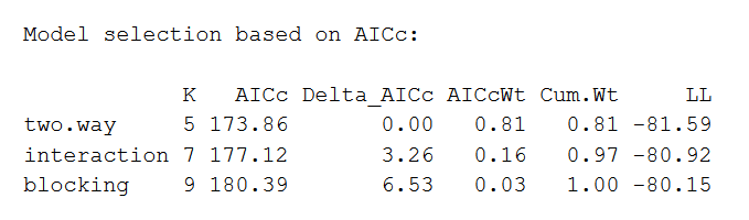
The AIC model with the best fit will be listed first, with the second-best listed next, and so on. This comparison reveals that the two-way ANOVA without any interaction or blocking effects is the best fit for the data.
Interpreting the results of a two-way ANOVA
You can view the summary of the two-way model in R using the summary() command. We will take a look at the results of the first model, which we found was the best fit for our data.
summary(two.way)The output looks like this:
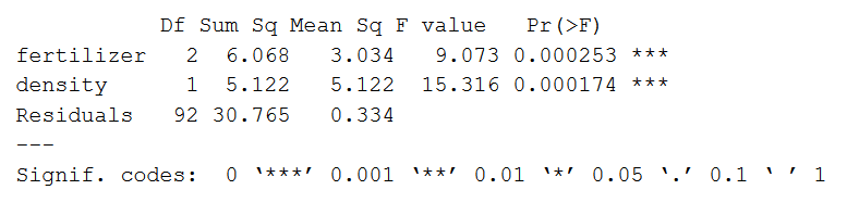
The model summary first lists the independent variables being tested (‘fertilizer’ and ‘density’). Next is the residual variance (‘Residuals’), which is the variation in the dependent variable that isn’t explained by the independent variables.
The following columns provide all of the information needed to interpret the model:
- Df shows the degrees of freedom for each variable (number of levels in the variable minus 1).
- Sum sq is the sum of squares (a.k.a. the variation between the group means created by the levels of the independent variable and the overall mean).
- Mean sq shows the mean sum of squares (the sum of squares divided by the degrees of freedom).
- F value is the test statistic from the F-test (the mean square of the variable divided by the mean square of each parameter).
- Pr(>F) is the p-value of the F statistic, and shows how likely it is that the F-value calculated from the F-test would have occurred if the null hypothesis of no difference was true.
From this output we can see that both fertilizer type and planting density explain a significant amount of variation in average crop yield (p-values < 0.001).
Post-hoc testing
ANOVA will tell you which parameters are significant, but not which levels are actually different from one another. To test this we can use a post-hoc test. The Tukey’s Honestly-Significant-Difference (TukeyHSD) test lets us see which groups are different from one another.
TukeyHSD(two.way)The output looks like this:
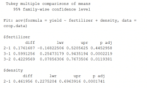
This output shows the pairwise differences between the three types of fertilizer ($fertilizer) and between the two levels of planting density ($density), with the average difference (‘diff’), the lower and upper bounds of the 95% confidence interval (‘lwr’ and ‘upr’) and the p-value of the difference (‘p-adj’).
From the post-hoc test results, we see that there are significant differences (p < 0.05) between:
- fertilizer groups 3 and 1,
- fertilizer types 3 and 2,
- the two levels of planting density,
but no difference between fertilizer groups 2 and 1.
How to present the results of a a two-way ANOVA
Once you have your model output, you can report the results in the results section of your paper.
When reporting the results you should include the f-statistic, degrees of freedom, and p-value from your model output.
A Tukey post-hoc test revealed significant pairwise differences between fertilizer mix 3 and fertilizer mix 1 (+ 0.59 bushels/acre under mix 3), between fertilizer mix 3 and fertilizer mix 2 (+ 0.42 bushels/acre under mix 2), and between planting density 2 and planting density 1 ( + 0.46 bushels/acre under density 2).
You can discuss what these findings mean in the discussion section of your paper.
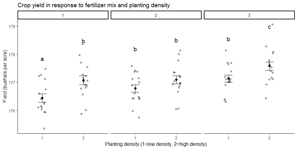
You may also want to make a graph of your results to illustrate your findings.
Your graph should include the groupwise comparisons tested in the ANOVA, with the raw data points, summary statistics (represented here as means and standard error bars), and letters or significance values above the groups to show which groups are significantly different from the others.
Frequently asked questions about two-way ANOVA
- What is the difference between a one-way and a two-way ANOVA?
-
The only difference between one-way and two-way ANOVA is the number of independent variables. A one-way ANOVA has one independent variable, while a two-way ANOVA has two.
- One-way ANOVA: Testing the relationship between shoe brand (Nike, Adidas, Saucony, Hoka) and race finish times in a marathon.
- Two-way ANOVA: Testing the relationship between shoe brand (Nike, Adidas, Saucony, Hoka), runner age group (junior, senior, master’s), and race finishing times in a marathon.
All ANOVAs are designed to test for differences among three or more groups. If you are only testing for a difference between two groups, use a t-test instead.
- How is statistical significance calculated in an ANOVA?
-
In ANOVA, the null hypothesis is that there is no difference among group means. If any group differs significantly from the overall group mean, then the ANOVA will report a statistically significant result.
Significant differences among group means are calculated using the F statistic, which is the ratio of the mean sum of squares (the variance explained by the independent variable) to the mean square error (the variance left over).
If the F statistic is higher than the critical value (the value of F that corresponds with your alpha value, usually 0.05), then the difference among groups is deemed statistically significant.
- What is a factorial ANOVA?
-
A factorial ANOVA is any ANOVA that uses more than one categorical independent variable. A two-way ANOVA is a type of factorial ANOVA.
Some examples of factorial ANOVAs include:
- Testing the combined effects of vaccination (vaccinated or not vaccinated) and health status (healthy or pre-existing condition) on the rate of flu infection in a population.
- Testing the effects of marital status (married, single, divorced, widowed), job status (employed, self-employed, unemployed, retired), and family history (no family history, some family history) on the incidence of depression in a population.
- Testing the effects of feed type (type A, B, or C) and barn crowding (not crowded, somewhat crowded, very crowded) on the final weight of chickens in a commercial farming operation.
- What is the difference between quantitative and categorical variables?
-
Quantitative variables are any variables where the data represent amounts (e.g. height, weight, or age).
Categorical variables are any variables where the data represent groups. This includes rankings (e.g. finishing places in a race), classifications (e.g. brands of cereal), and binary outcomes (e.g. coin flips).
You need to know what type of variables you are working with to choose the right statistical test for your data and interpret your results.
Sources in this article
We strongly encourage students to use sources in their work. You can cite our article (APA Style) or take a deep dive into the articles below.
This Scribbr articleBevans, R. (October 3, 2022). Two-Way ANOVA | Examples & When To Use It. Scribbr. Retrieved October 17, 2022, from https://www.scribbr.com/statistics/two-way-anova/
